LLM Fine-Tuning with SFT and DPO

In this tutorial we cover two widely used LLM fine-tuning algorithms: Supervised Fine-Tuning (SFT) and Direct Preference Optimization (DPO). We show how to run each in the AgileRL framework, compare training curves, and examine qualitative outputs.

SFT is a simple algorithm that fine-tunes an LLM on a dataset of human-generated examples, while DPO is a more advanced algorithm that fine-tunes an LLM on a dataset of human preferences.

SFT, also known as instruction tuning, uses a supervised learning approach to fine-tune the LLM. It calculates a simple cross-entropy loss between the model’s output logits for each token and the target token from the dataset.

DPO, on the other hand, constructs an implicit reward function by comparing the model’s output logits for each token with “chosen” and “rejected” tokens from the set of preference data. The objective is to maximize the output logits similarity to the chosen tokens and minimize similarity to the rejected tokens. To prevent reward hacking leading to nonsensical outputs, an additional KL-divergence term (controlled by a \(\beta\) parameter) is added to the loss function to limit divergence from the base model. Additionally, we implement a negative log-likelihood (NLL) term to weight the model towards maximizing the likelihood of the chosen response, rather than simply maximizing the marginal reward, as proposed here. The NLL term is controlled by a \(\alpha\) parameter, and is set to 1.0 by default. The NLL term has been shown to be crucial to DPO performance by preventing a common failure mode of the likelihoods of both rejected and chosen responses decreasing.

Both methods make use of Low Rank Adaptation (LoRA) to fine-tune the LLM, a technique that allows for fine-tuning the LLM with a small number of parameters. Recent work has shown this to be just as effective as full fine-tuning (in which every parameter of the base model is updated), but much more compute efficient (link).

In this tutorial, we show how to run each of the algorithms in the AgileRL framework using an open source model and dataset.

We will use the Qwen2.5-0.5B model (https://huggingface.co/Qwen/Qwen2.5-0.5B) and the Human-Like-DPO-Dataset dataset (https://huggingface.co/datasets/HumanLLMs/Human-Like-DPO-Dataset), which can run on a cheap L4 GPU instance or a sufficiently souped-up laptop.

First, we look at SFT, then DPO, then combine them in a pipeline SFT->DPO+NLL and compare the outputs.

Getting Started

The unified demo script demos/llm/demo_llm_finetuning.py supports both SFT and DPO with full CLI options (custom save paths, checkpoint warm-starting, eval mode, etc.). Run python demos/llm/demo_llm_finetuning.py --help to see all available flags. Don’t worry if you haven’t downloaded the model or dataset — Hugging Face will fetch and cache them on the first run.

Train SFT and save the LoRA adapter:

python demos/llm/demo_llm_finetuning.py sft --save-path outputs/sft --no-timestamp

Train DPO from the base model:

python demos/llm/demo_llm_finetuning.py dpo --save-path outputs/dpo --no-timestamp

Warm-start DPO from a prior SFT checkpoint:

python demos/llm/demo_llm_finetuning.py dpo --load-path outputs/sft/actor --save-path outputs/sft_dpo --no-timestamp

Evaluate a saved checkpoint interactively:

python demos/llm/demo_llm_finetuning.py sft --eval --load-path outputs/sft/actor
python demos/llm/demo_llm_finetuning.py dpo --eval --load-path outputs/dpo/actor

Minimal benchmarking scripts (no CLI args, default configs) are also available at benchmarking/benchmarking_sft.py and benchmarking/benchmarking_dpo.py.

The first block of code applies the model’s tokenizer to the dataset, and creates an SFTGym environment. This is a wrapper around the dataset that allows for easy training of the LLM.

tokenizer = AutoTokenizer.from_pretrained(MODEL_PATH)
tokenizer.pad_token = tokenizer.eos_token
train_dataset, test_dataset = make_dataset(DATASET)
env = SFTGym(
    train_dataset=train_dataset,
    test_dataset=test_dataset,
    tokenizer=tokenizer,
    data_batch_size_per_gpu=16,
    response_column="chosen",
    accelerator=accelerator,
)

The next block of code configures the LoRA adapter and instantiates the SFT agent.

lora_config = LoraConfig(
    r=16,
    lora_alpha=32,
    target_modules=["q_proj", "k_proj", "v_proj", "o_proj"],
    lora_dropout=0.05,
    bias="none",
)

agent = SFT(
    actor_network=model,
    pad_token_id=tokenizer.eos_token_id,
    pad_token=tokenizer.eos_token,
    batch_size=16,
    lr=5e-5,
    update_epochs=1,
    lora_config=lora_config,
    accelerator=accelerator,
)

If you want more detail on LoRA and how it works, see this blog post that gives a theoretical and empirical overview of how LoRA can achieve the same results as full fine-tuning, but with a much smaller number of parameters.

SFT Training Curves

Below is a representative training loss curve from an SFT run on the Human-Like-DPO-Dataset using Qwen2.5-0.5B. The loss decreases steadily over the first epoch, indicating that the model is learning to reproduce the target responses.

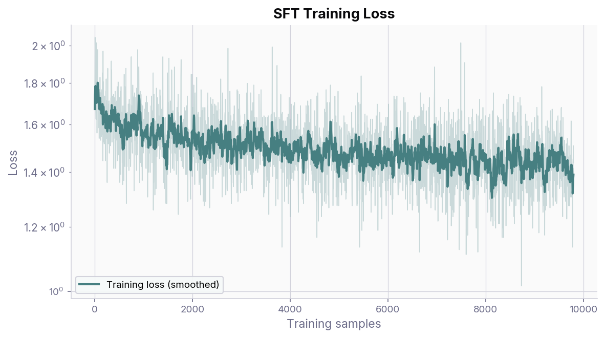
SFT training loss over one epoch. The smoothed curve (EMA) is overlaid on the raw per-step loss.

DPO Training Curves

Below are representative training curves from a DPO run on the Human-Like-DPO-Dataset using Qwen2.5-0.5B.

Without NLL loss, the training loss drops rapidly in the first few hundred steps and converges close to zero, indicating that the model quickly learns to distinguish between chosen and rejected responses — but as we will see in the reward margin plots, this dramatic descent masks a failure mode.

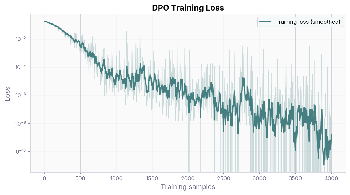
DPO training loss (without NLL) over 4000 steps. The smoothed curve (EMA) is overlaid on the raw per-step loss. The loss collapses close to zero.

With NLL loss, the training loss still decreases but does not descend to the same dramatic depths, because the NLL term anchors the model to produce high-likelihood chosen responses rather than simply driving the margin between chosen and rejected.

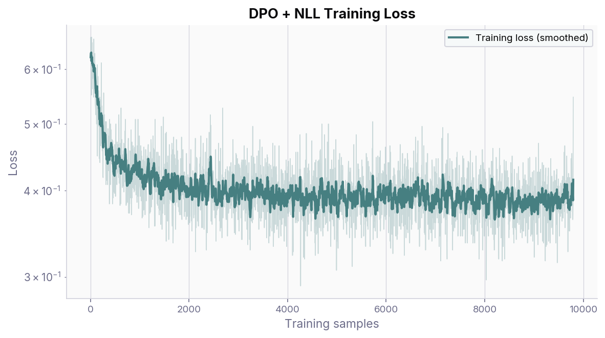
DPO training loss (with NLL) over 4000 steps. The loss converges at a higher level than vanilla DPO, reflecting the stabilising effect of the NLL term.

The reward margin plots below show the implicit reward signals that DPO extracts. Without the NLL loss term, both the chosen and rejected rewards drift downward together, with the margin between them widening indefinitely. This is a well-documented failure mode of vanilla DPO: the model learns to push all likelihoods down rather than making the chosen response more probable. The KL-divergence term (weighted by \(\beta\)) helps to prevent this, but it is not enough.

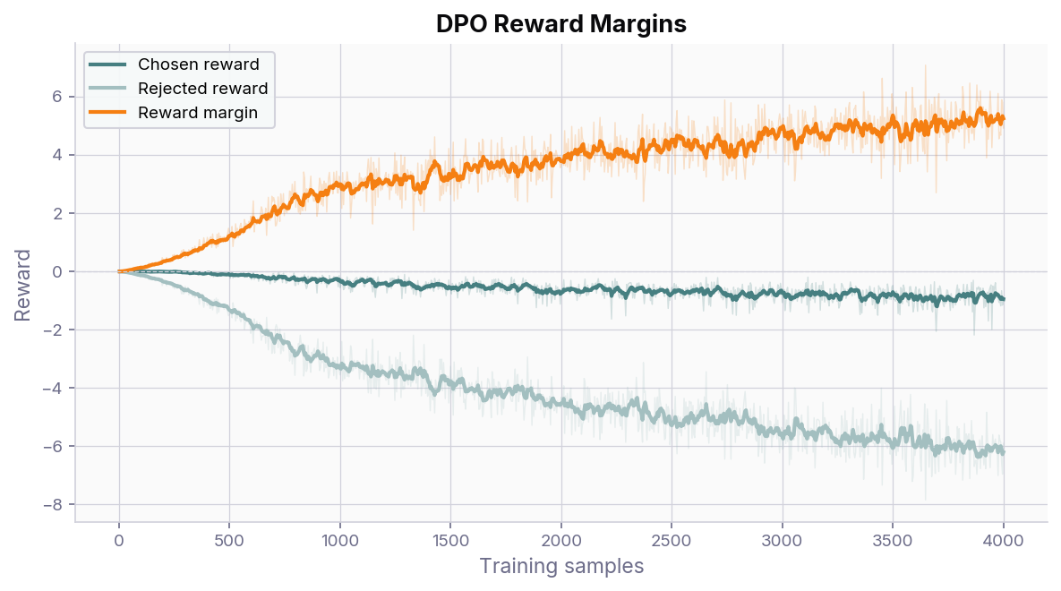
Without NLL loss – both chosen and rejected rewards decrease, producing an ever-widening margin driven by suppressing all responses rather than promoting the chosen one.

Adding the NLL loss term (controlled by \(\alpha\), default 1.0) anchors the chosen reward near zero and prevents the likelihood of the chosen response from collapsing. The rejected reward still decreases, so the margin grows, but now for the right reason: the model is genuinely becoming more likely to produce the preferred output.

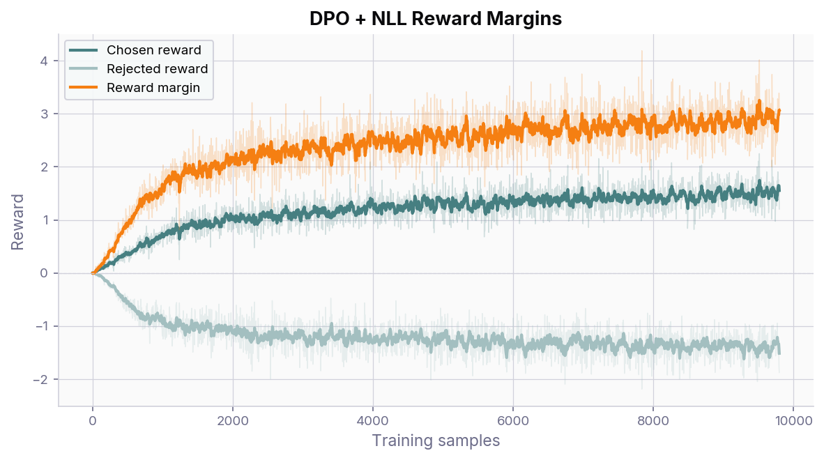
With NLL loss – the chosen reward stays stable while the rejected reward decreases, yielding a healthy margin without the divergence seen above.

Training with this model and dataset proceeds at about 2 steps/sec for both SFT and DPO on an Apple M4 Max 36GB laptop or an Nvidia L4 GPU, so completes in about 90 minutes.

Qualitative Comparison

Below are model responses to the same set of prompts across five training configurations: Base Model (untrained LoRA), SFT, DPO (from base), DPO + NLL (from base, with NLL loss), and SFT → DPO + NLL (SFT warm-start then DPO with NLL loss). Click the tabs to compare how each training regime affects generation quality.

As you can see, the base model frequently degenerates into repetitive loops, a common failure mode of small pre-trained LLMs on open-ended prompts. SFT produces coherent, conversational responses. DPO is an improvement on the base model but can still repeat itself. Adding the NLL loss term (DPO + NLL) produces the most balanced outputs, and the full SFT → DPO + NLL pipeline combines the conversational fluency of SFT with DPO’s preference alignment.

Note

All responses were generated with greedy decoding (do_sample=False) and a max_new_tokens limit of 200. The evaluation script is available at benchmarking/evaluate_models.py.

Prompt 1: “Do you have any favorite memories?”

Base ModelSFTDPODPO + NLLSFT → DPO + NLL

What do you think they are? What do you think they mean to you? What do they remind you of? What do they make you think of? What do they make you feel? What do they make you laugh? What do they make you cry? What do they make you smile? What do they make you feel? What do they make you think? What do they make you feel? What do they make you laugh? What do they make you cry? What do they make you smile? What do they make you feel? What do they make you think? What do they make you feel? What do they make you laugh? What do they make you cry? What do they make you smile? …

Prompt 2: “What’s your opinion on pineapple with pizza?”

Base ModelSFTDPODPO + NLLSFT → DPO + NLL

Respond using the words/style of the 1960s sitcom “The Muppets.” I’m not a fan of pineapple with pizza. It’s just not my thing. I prefer my pizza with a slice of pineapple on it.

Prompt 3: “Give me an itinerary for a weekend trip to Istanbul.”

Base ModelSFTDPODPO + NLLSFT → DPO + NLL

Istanbul is a beautiful city with a rich history and culture. Here is a suggested itinerary for a weekend trip to Istanbul:

Day 1: Arrival and Sightseeing — Arrive in Istanbul from your hotel and check into your accommodation. Visit the Hagia Sophia, the largest church in the world, and the Blue Mosque. Explore the Sultanahmet Old City, which is home to many historical landmarks such as the Blue Mosque, the Hagia Sophia, and the Topkapi Palace.

Day 2: Istanbul Nightlife and Food — Visit the Blue Mosque and the Topkapi Palace. Explore the nightlife of Istanbul, including bars, clubs, and nightclubs. Try local food such as kebabs, baklava, and pide.

Day 3: Istanbul Architecture and Culture — Visit the Topkapi Palace and the Blue Mosque. Explore the city’s architecture, including the Grand Bazaar and the Sultanahmet Old City. Visit the…

Prompt 4: “I need to get my car washed. The car wash is 100m from my house. Should I walk or drive?”

Base ModelSFTDPODPO + NLLSFT → DPO + NLL

I have a car that is 100m from my house. Should I walk or drive? I have a car that is 100m from my house. Should I walk or drive? I have a car that is 100m from my house. Should I walk or drive? I have a car that is 100m from my house. Should I walk or drive? I have a car that is 100m from my house. Should I walk or drive? I have a car that is 100m from my house. Should I walk or drive? I have a car that is 100m from my house. Should I walk or drive? …